Dr. Ge Wang is grateful for valuable suggestions from Drs. Michael Vannier, Tiange Zhuang, and others, as well as the Rensselaer Polytechnic Institute. Watch Dr. Wang's talk on computed tomography to learn more about this topic.

To quantify the interaction between X-rays and matter, first we take a piece of material with a small thickness, T. Then, let an X-ray source send N photons to the material sample. Due to the attenuation effect, there will be a small loss, Δ, in the number of X-ray photons through the sample. Hence, the number of X-ray photons recorded by an X-ray detector behind the sample is N-Δ. The thicker the element thickness T, the greater the loss Δ; and the larger the number of incoming photons N, the greater the loss Δ. A good approximation is that Δ=μTN, where μ is the attenuation coefficient. In other words, given N, T and Δ, we can easily find μ, which reflects how strongly the material blocks X-rays.

If there are a series of material elements along an X-ray path, the X-ray beam will be sequentially attenuated by these elements. The total loss in the number of X-ray photons will be the sum of contributions made by all the involved elements. With a data processing step, we can find the sum of attenuation coefficients associated with these elements from the number of incoming X-ray photons and the number of recorded X-ray photons. In other words, with a pencil X-ray beam we can probe into an object to obtain the sum of attenuation coefficients of material elements along an X-ray path.

A cross-sectional image is an array of attenuation coefficients, with each material element defining an image pixel (picture element). What we measure with X-rays are sums of attenuation coefficients along various paths. What we desire to have for visualization are individual attenuation coefficients in a matrix format to form an image. Then, the question is how to find individual coefficients from their sums along different paths?

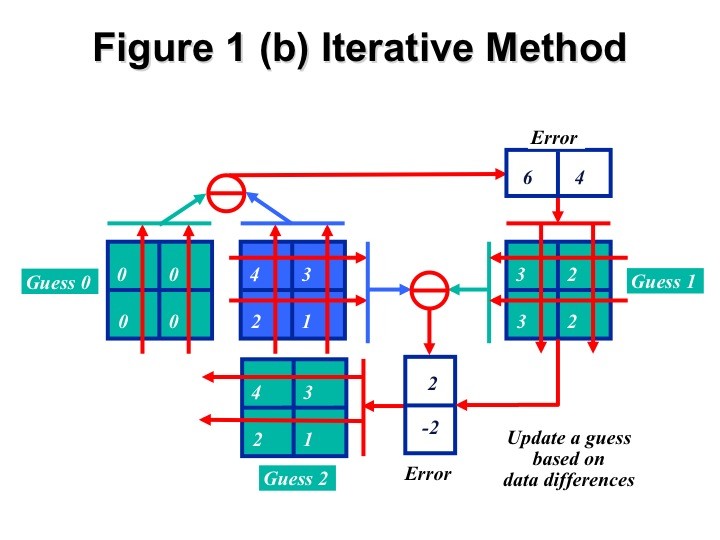
If we have a 2 by 2 matrix containing four unknowns, we can form two horizontal paths to cover this matrix. Additionally, we can have two vertical paths to do the same. The sums along these four paths give four equations. From four equations of four unknowns, we can often solve for a solution, as illustrated in Figure 1. Indeed, we can do so using an iterative method, via trial and error. For example, starting from a zero-valued matrix as an initial guess, we can construct two vertical sums through the guessed matrix, and compare the resultant sums with the real counterparts. Then, the differences are uniformly put back along the vertical paths to update the guess so that there will be no errors between the sums based on the updated guess and those measured from the real image. With the updated guess, we can form two horizontal sums, and compare them with the real counterparts. Similarly, the differences are uniformly put back along the involved paths to update the guess so that there will be no errors between the predicted and measured sums. This second iteration reconstructs the 2 by 2 image correctly! In practice, an image matrix is much larger, and many updating steps are needed.

Figure 1. Image reconstruction through equation solving. A system of four equations (Left) can be solved using an iterative method (Right).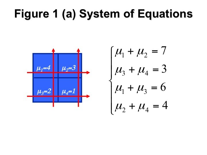Actually, the combination of two horizontal and two vertical paths we just used is not the best design because one of the equations can be derived from the other three.. To make sure we have a unique solution, we can replace a vertical ray with a diagonal ray for four independent equations. In principle, we can always have a design to get as many independent measures as needed.

Figure 2 gives a complementary perspective. Let us decompose an image into triangular elements (instead of square pixels as before) formed by recursively inscribed regular hexagons. Each triangular element is assumed to be homogeneous. First, we can directly measure the most peripheral triangular elements (in red) with X-rays and compute their attenuation coefficients (as explained earlier). Then, we can handle the elements in the next layer (in green). An X-ray beam through a green element also intersects two red elements that are already known at this stage. Thus, the known attenuation coefficient of the green element can be directly computed after the coefficients for the involved red elements are taken into account. So on and so forth (when a hexagon becomes small enough, it can be decomposed into four small triangles) until all the attenuation coefficients of the triangular elements are found.
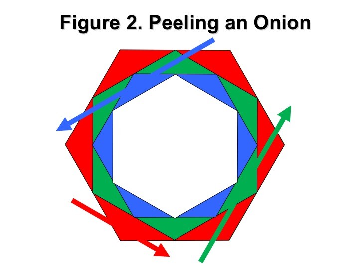Figure 2. Image reconstruction via “onion-peeling”. Attenuation coefficients of the triangular elements can be determined layer-by-layer towards the center.

Next Section »